ZeRO: Zero Redundancy Optimizer

When you train large models with data parallelism, every GPU holds a full copy of everything. The model parameters, the gradients, the optimizer states. All of it, duplicated on every single GPU. Most of that memory is wasted. ZeRO gets rid of this waste by splitting these states across GPUs instead of copying them.

Think of it like a group project where everyone prints the entire textbook. ZeRO says: just split the chapters, and share when needed.

Papers:

ZeRO: Memory Optimizations Toward Training Trillion Parameter Models (Rajbhandari et al., 2019)

ZeRO-Offload: Democratizing Billion-Scale Model Training (Ren et al., 2021)

ZeRO-Infinity: Breaking the GPU Memory Wall for Extreme Scale Deep Learning (Rajbhandari et al., 2021)

---

The Memory Problem

Say you have a model with $\Psi$ parameters. You train it with Adam in mixed precision, so you keep fp16 parameters for the forward/backward pass and fp32 copies for the optimizer. Let’s count the bytes per GPU:

The fp16 parameters take $2\Psi$ bytes. The fp16 gradients take another $2\Psi$ bytes. Then Adam needs three fp32 tensors: a master copy of the parameters ($4\Psi$), the momentum ($4\Psi$), and the variance ($4\Psi$). That gives us:

$\text{Total per GPU} = 2\Psi + 2\Psi + 4\Psi + 4\Psi + 4\Psi = 16\Psi$

The optimizer states alone eat $12\Psi$ bytes. That is 75% of the memory. And with standard data parallelism, every GPU stores all $16\Psi$ bytes. If you have 64 GPUs, you are storing 64 identical copies of those optimizer states. That is the redundancy ZeRO targets.

---

Notation

We will use these symbols throughout the post:

$\Psi$ is the number of model parameters.

$N_d$ is the data parallelism degree (number of GPUs).

$P_{os}$ refers to optimizer state partitioning (Stage 1).

$P_{os+g}$ refers to optimizer state and gradient partitioning (Stage 2).

$P_{os+g+p}$ refers to full partitioning of optimizer states, gradients, and parameters (Stage 3).

---

The Three Stages

ZeRO partitions memory across $N_d$ GPUs in three progressive stages. Each one removes more redundancy.

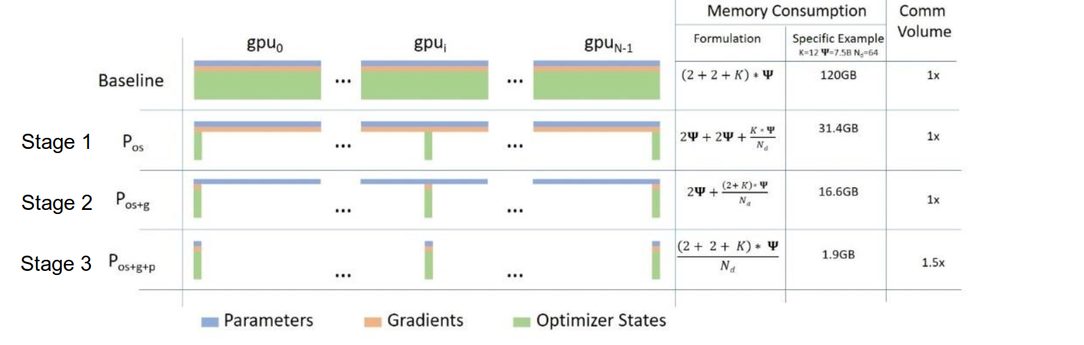
Stage 1: Partition Optimizer States ($P_{os}$)

Instead of every GPU holding all optimizer states, we shard them. Each GPU owns optimizer states for only $\frac{\Psi}{N_d}$ parameters.

The memory per GPU becomes:

$M_{\text{stage1}} = 2\Psi + 2\Psi + \frac{12\Psi}{N_d} = 4\Psi + \frac{12\Psi}{N_d}$

The first $2\Psi$ is the fp16 parameters (still fully replicated). The second $2\Psi$ is the fp16 gradients (also fully replicated). The $\frac{12\Psi}{N_d}$ is the optimizer shard, each GPU only stores its chunk.

With 64 GPUs, that goes from $16\Psi$ down to roughly $4.2\Psi$. A 4x reduction.

Each GPU still runs the full forward and backward pass, so it computes gradients for all parameters. But it only runs Adam on its own shard. After the update, an all-gather sends the updated parameters back to everyone.

Stage 2: Partition Gradients ($P_{os+g}$)

If a GPU only updates its own shard of the optimizer, why keep gradients for parameters it does not own? Stage 2 removes this waste.

Each GPU only stores gradients for the parameters whose optimizer states it owns. Gradients for other parameters get reduce-scattered to the owning GPU and thrown away.

Memory per GPU:

$M_{\text{stage2}} = 2\Psi + \frac{2\Psi}{N_d} + \frac{12\Psi}{N_d} = 2\Psi + \frac{14\Psi}{N_d}$

Now only the fp16 parameters ($2\Psi$) are fully replicated. Everything else is sharded. With 64 GPUs this is roughly $2.2\Psi$, an 8x reduction.

Stage 3: Partition Parameters ($P_{os+g+p}$)

Everything is sharded. Each GPU only stores $\frac{\Psi}{N_d}$ parameters. When a layer needs the full parameters for forward or backward, it collects them on the fly with an all-gather, uses them, then throws away the parts it does not own.

Memory per GPU:

$M_{\text{stage3}} = \frac{2\Psi}{N_d} + \frac{2\Psi}{N_d} + \frac{12\Psi}{N_d} = \frac{16\Psi}{N_d}$

With 64 GPUs: $\frac{16\Psi}{64} = 0.25\Psi$. A 64x reduction that scales linearly with GPU count.

---

Communication Cost

The natural question is: does all this sharding make communication more expensive?

Standard data parallelism uses an all-reduce to sync gradients, which costs $2\Psi$ per GPU. Stages 1 and 2 have the exact same communication cost because an all-reduce is really just a reduce-scatter followed by an all-gather:

$\text{all-reduce} = \text{reduce-scatter} + \text{all-gather}$

ZeRO does the same two operations. It just keeps less data around between them. So Stages 1 and 2 cost $2\Psi$, same as vanilla data parallelism. No extra overhead.

Stage 3 costs $3\Psi$ because parameters need to be collected before both the forward and backward pass. That is $\Psi$ for the forward all-gather, $\Psi$ for the backward all-gather, and $\Psi$ for the reduce-scatter. A 1.5x increase over standard DP, which is a small price for the memory savings.

---

Stage 1 Deep Dive: Optimizer State Partitioning

This is the simplest stage and gives you the biggest win for the least effort. Let’s walk through how it works.

Standard Data Parallelism

In normal data parallelism with Adam, the training loop looks like this:

1. Forward. Each GPU runs the forward pass on its mini-batch. All GPUs have the full model.
2. Backward. Each GPU computes gradients for all parameters.
3. All-reduce. Average the gradients across all GPUs.
4. Update. Every GPU runs Adam on all $\Psi$ parameters.

Step 4 is pure waste. Every GPU does the exact same Adam computation and stores the exact same optimizer states. It is like every person in a team doing the same calculation independently and getting the same answer.

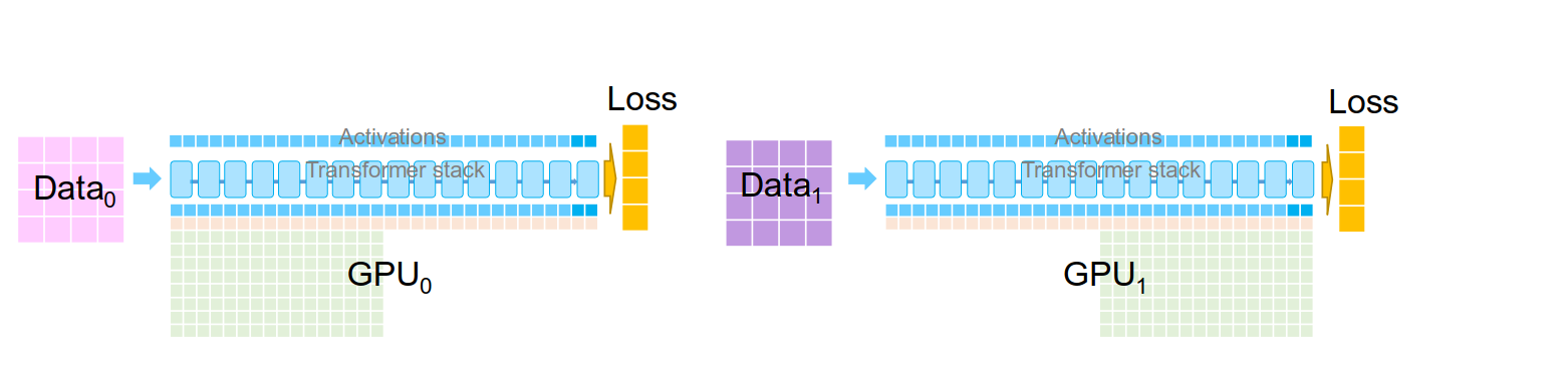
ZeRO Stage 1

ZeRO Stage 1 changes step 4 by splitting the work:

1. Forward. Same as before, full model on each GPU.
2. Backward. Same as before, full gradients on each GPU.
3. Reduce-scatter. Each GPU receives the averaged gradient only for its shard.
4. Update. Each GPU runs Adam only on its $\frac{\Psi}{N_d}$ parameters.
5. All-gather. Broadcast updated parameters so every GPU has the full model again.

Flat Partitioning

The parameters are split into $N_d$ contiguous chunks. We flatten all parameters into one big 1D tensor and divide it evenly. GPU $i$ owns chunk $i$:

$\text{GPU}_i \text{ owns parameters } \left[\frac{i \cdot \Psi}{N_d}, \;\frac{(i+1) \cdot \Psi}{N_d}\right)$

This flat split is simpler than partitioning by layer and gives perfect load balance.

The Collectives

In standard DP, the all-reduce that syncs gradients is equivalent to a reduce-scatter followed by an all-gather. ZeRO Stage 1 takes advantage of this. Instead of doing the full all-reduce and then having every GPU update all parameters, we split it:

First, reduce-scatter the gradients. Each GPU $i$ ends up with the averaged gradient only for its shard. Then each GPU runs Adam locally on its shard. Finally, all-gather the updated parameters so every GPU has the full model.

The total communication is still $2\Psi$. We just inserted the optimizer step between the two halves of the all-reduce.

Why It Gives the Same Result

Let $g_n^{(k)}$ be the gradient of parameter $n$ on GPU $k$. Standard DP computes the average gradient on every GPU:

$\bar{g}_n = \frac{1}{N_d} \sum_{k=0}^{N_d - 1} g_n^{(k)}$

Then every GPU applies Adam:

$\theta_n \leftarrow \text{Adam}(\theta_n, \bar{g}_n)$

ZeRO Stage 1 computes $\bar{g}_n$ only on the GPU that owns parameter $n$, applies Adam there, and broadcasts the updated $\theta_n$ back. The final result is identical. We just avoided storing Adam’s momentum $m_n$ and variance $v_n$ on GPUs that do not own parameter $n$.

Memory Breakdown

Before ZeRO (standard DP), each GPU stores:

$\underbrace{2\Psi}_{\text{fp16 params}} + \underbrace{2\Psi}_{\text{fp16 grads}} + \underbrace{4\Psi}_{\text{fp32 master}} + \underbrace{4\Psi}_{m_n} + \underbrace{4\Psi}_{v_n} = 16\Psi$

After Stage 1, the three optimizer tensors (master copy, momentum, variance) are divided by $N_d$:

$\underbrace{2\Psi}_{\text{fp16 params}} + \underbrace{2\Psi}_{\text{fp16 grads}} + \underbrace{\frac{12\Psi}{N_d}}_{\text{optimizer shard}} = 4\Psi + \frac{12\Psi}{N_d}$

Parameters and gradients are still fully replicated. Stage 1 only touches the optimizer states.

---

Stage 2 Deep Dive: Gradient Partitioning

Stage 1 still keeps full gradients on every GPU. But if GPU $i$ only runs Adam on its shard, it does not need gradients for parameters it does not own. Stage 2 removes them.

How It Works

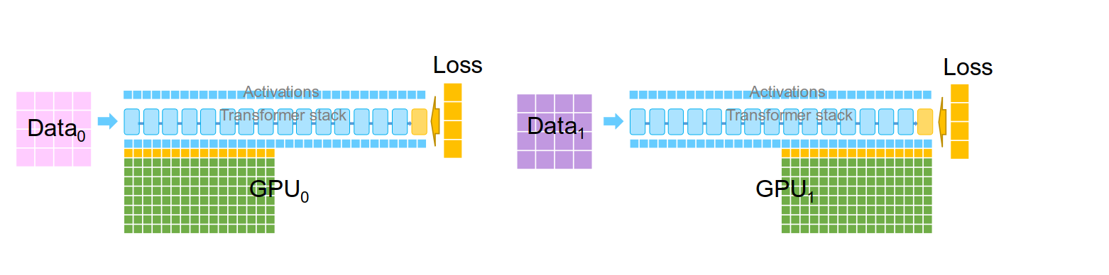
During the backward pass, as gradients are computed layer by layer, we immediately reduce-scatter them. Each GPU only keeps the averaged gradient for its own shard. Gradients for other shards get sent to their owners and discarded right away.

The training loop becomes:

1. Forward. Full model on each GPU.
2. Backward + reduce-scatter. As each layer’s gradients are computed, reduce-scatter them. Each GPU keeps only its shard’s gradients.
3. Update. Each GPU runs Adam on its shard.
4. All-gather. Broadcast updated parameters.

Overlapping Communication with Computation

The key trick in Stage 2 is gradient bucketing. We do not wait for the entire backward pass to finish before communicating. Gradients are grouped into buckets, which are contiguous chunks of memory. As soon as a bucket is full (all its gradients have been computed), we launch the reduce-scatter for that bucket while the backward pass keeps computing gradients for later layers.

Think of it like an assembly line. One worker is still building products while the previous batch is already being shipped out. The communication is almost fully hidden behind the backward computation.

Memory

We drop $2\Psi$ of gradient storage down to $\frac{2\Psi}{N_d}$:

$M_{\text{stage2}} = \underbrace{2\Psi}_{\text{fp16 params}} + \underbrace{\frac{2\Psi}{N_d}}_{\text{grad shard}} + \underbrace{\frac{12\Psi}{N_d}}_{\text{optimizer shard}} = 2\Psi + \frac{14\Psi}{N_d}$

Communication stays at $2\Psi$. We are still doing one reduce-scatter and one all-gather, same as Stages 1 and standard DP.

---

Stage 3 Deep Dive: Parameter Partitioning

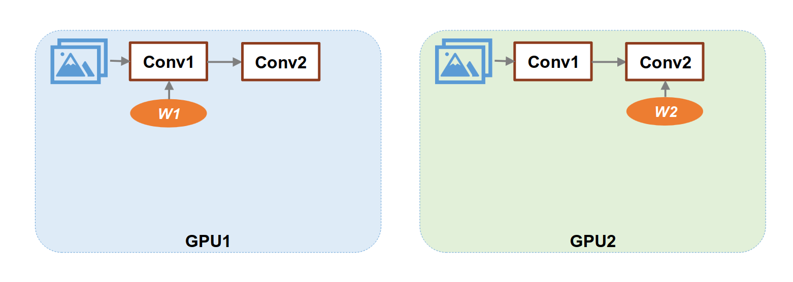
Stage 3 goes all the way. Even the model parameters are sharded. Each GPU only stores $\frac{\Psi}{N_d}$ parameters.

The Challenge

If GPU $i$ only holds a fraction of the parameters, how does it run the forward pass? A layer needs all its parameters to compute its output.

All-Gather on Demand

The solution is simple: before computing a layer, we all-gather its full parameters from all GPUs. After using them, we throw away the parts we do not own.

During the forward pass, for each layer $l$: all-gather the full parameters for layer $l$, compute the forward pass, then discard the non-owned parameters.

During the backward pass, same thing in reverse order: all-gather the full parameters for layer $l$ again, compute the backward pass, reduce-scatter the gradients to owners, then discard the non-owned parameters.

After backward, each GPU runs Adam on its shard. No final all-gather is needed because the parameters are already where they belong.

It is like a library with one copy of each book shared between all readers. When you need a book, you borrow it, read the chapter you need, and return it. You do not keep a personal copy.

The Extra Communication

Stages 1 and 2 do one all-gather per training step (after the optimizer update). Stage 3 does two all-gathers, one in forward and one in backward, plus the reduce-scatter:

$\text{Stage 3 comm} = \underbrace{\Psi}_{\text{all-gather (fwd)}} + \underbrace{\Psi}_{\text{all-gather (bwd)}} + \underbrace{\Psi}_{\text{reduce-scatter}} = 3\Psi$

That is 1.5x the cost of standard DP. But memory scales as $\frac{16\Psi}{N_d}$, perfectly linear with the number of GPUs.

When You Need Stage 3

Stage 3 is necessary when the model itself does not fit on a single GPU. A 10B parameter model needs 20GB just for fp16 parameters. With Stage 3 across 8 GPUs, each GPU holds only 2.5GB of parameters. The 1.5x communication cost is worth it because without Stage 3 you simply cannot train the model with pure data parallelism.

---

ZeRO-Offload and ZeRO-Infinity

The original ZeRO partitions across GPUs. The follow-up papers extend this idea to different types of memory.

ZeRO-Offload

ZeRO-Offload moves optimizer states and optionally gradients to CPU memory. CPU RAM is much larger than GPU memory, so this lets you train bigger models on fewer GPUs.

The forward and backward passes stay on the GPU. Only the optimizer step happens on the CPU. Gradients are reduced on GPU, sent to the CPU for the Adam update, and the updated parameters are copied back. The tradeoff is PCIe bandwidth, since CPU-GPU transfers are slower than GPU-GPU NVLink. But ZeRO-Offload is designed to minimize these transfers by only offloading the optimizer step, which is the least compute-intensive part of training.

ZeRO-Infinity

ZeRO-Infinity takes this further by offloading to NVMe SSDs on top of CPU memory. This breaks the memory wall entirely. You can train models limited only by disk space.

Parameters, gradients, and optimizer states can all live on NVMe. A prefetching system moves data from NVMe to CPU to GPU just in time for when it is needed, and overlaps these transfers with computation so the GPU is rarely waiting.

On a single DGX-2 node with 16 GPUs, ZeRO-Infinity can handle models with tens of trillions of parameters.

---

Summary

	Memory per GPU	Communication	What changes
Standard DP	$16\Psi$	$2\Psi$	Nothing partitioned
Stage 1	$4\Psi + \frac{12\Psi}{N_d}$	$2\Psi$	Optimizer states sharded
Stage 2	$2\Psi + \frac{14\Psi}{N_d}$	$2\Psi$	+ gradients sharded
Stage 3	$\frac{16\Psi}{N_d}$	$3\Psi$	+ parameters sharded

ZeRO’s insight is simple. Data parallelism replicates everything, but it only needs to replicate the computation. The states can be partitioned without changing the math. You just need the right communication primitives at the right time.

In the next parts we will implement each stage in code, starting with Stage 1.

---

References

[1] Rajbhandari, S., Rasley, J., Rabe, O., He, Y. (2019). ZeRO: Memory Optimizations Toward Training Trillion Parameter Models. arXiv:1910.02054

[2] Ren, J., Rajbhandari, S., Aminabadi, R.Y., Ruwase, O., Yang, S., Zhang, M., Li, D., He, Y. (2021). ZeRO-Offload: Democratizing Billion-Scale Model Training. arXiv:2101.06840

[3] Rajbhandari, S., Ruwase, O., Rasley, J., Smith, S., He, Y. (2021). ZeRO-Infinity: Breaking the GPU Memory Wall for Extreme Scale Deep Learning. arXiv:2104.07857

[4] Jia, Z. (2024). ML Parallelization (Part 1). CMU 15-779 Lecture Slides. PDF